library(BayesFR)
library(brms)
library(ggplot2)
library(bayesplot) # plotting posterior distributions
library(cowplot)   # ggplot grids
library(invgamma) # additional prior distribution10. Priors
Many people are insecure about choosing priors in Bayesian statistics, but there is no need to be! A very old-school approach on priors was a rule that they should be chosen before even looking at the data. A more modern approach is that we can test even “weakly informative” or “vague” priors and check if they are compatible with observations. This approach is strongly supported in the textbook “Statistical Rethinking” (McElreath, 2020). See also Wesner & Pomeranz (2021) for examples of ecological models, where non-informative priors are not always the best choice. In nonlinear models, this becomes even more important, since it is often hard to tell right away if a parameter’s prior is just weakly informative, or if it introduces a strong bias towards predictions that are widely out of the range of observed data.
Prior predictive checks are performed effortlessly in brms, simply by running a model fit specifying sample_prior="only". Here, MCMC samples only from the prior distributions, without taking the data into account. So the “fitted” model is not actually a model fit, and the samples from the “posterior distribution” are actually the prior distribution. These are used to compare predictions with observed data, i.e. using pp_check(), and plotting fitted and predicted distributions vs. observations with conditional_effects().
In this tutorial, we will first discuss exponential distributions as used frequently in the other tutorials. They are a quick choice for vague, or weakly informative positive priors. Second, we look into the gamma distribution, which through an additional scale parameter offers the choice of more informative positive priors. Third we discuss a reparameterization of the functional response using maximum feeding rate and half-saturation density, which can make prior choice a bit more straightforward if needed, especially for type 3 models.
data(df_Hossie_and_Murray_2010_OECOLOGIA)
df = subset(df_Hossie_and_Murray_2010_OECOLOGIA, ID=="Figure 1e")
ggplot(aes(N0,NE), data=df) +
  geom_jitter(width=0.1, height=0.0, alpha=0.6, size=2.5) +
  coord_cartesian(xlim=c(0,NA), ylim=c(0,NA))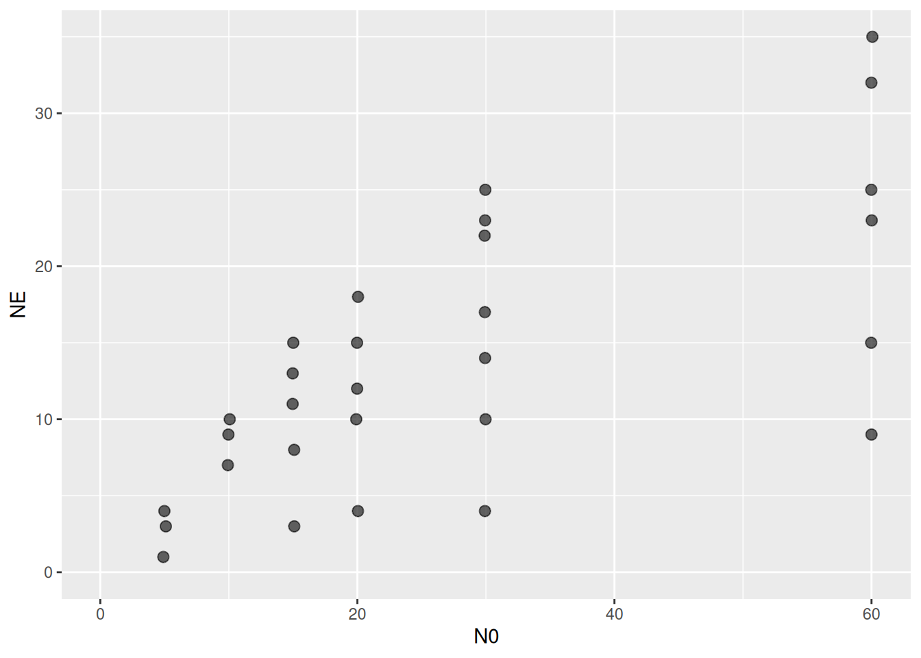
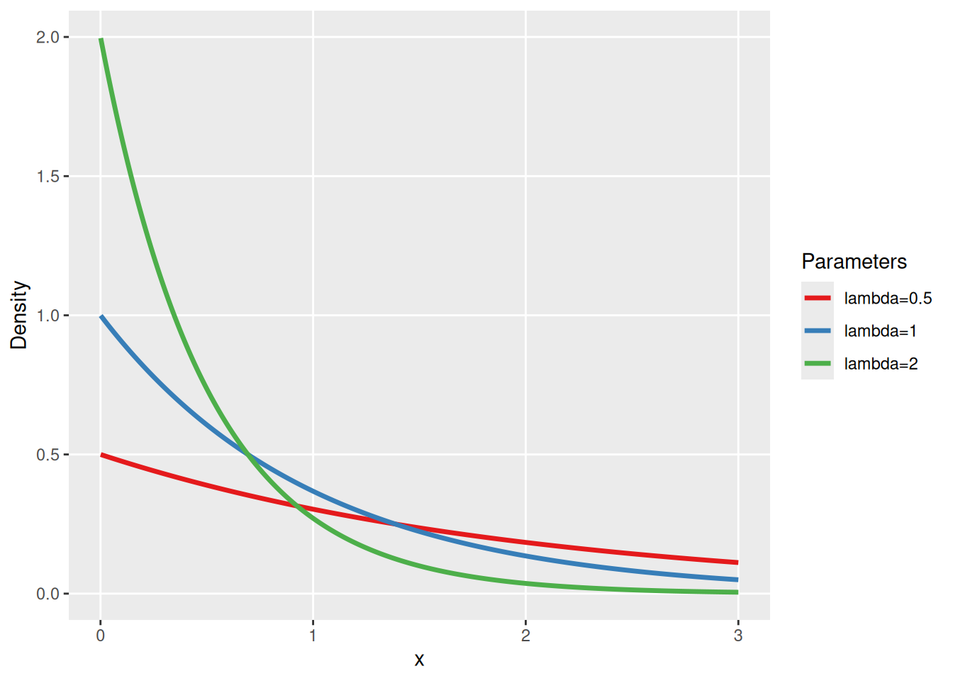
Weak priors: exponential distribution
The exponential distribution just has 1 parameter (rate \(\lambda\)), with mean and also variance given by its inverse \(1/ \lambda\). Hence, it is not possible to specify an independent level of information / certainty for a given mean.
Prior predictive check 1
We start by testing a naive prior choice for positive parameters \(a\) and \(h\) (rate \(\lambda=1.0\)).
FR.formula = bf( NE | trials(N0) ~ Type2H_dyn(N0,1.0,1.0,a,h)/N0,
                 a~1, h~1,
                 nl = TRUE)
FR.priors  = c(prior(exponential(1.0), nlpar="a", lb=0),
               prior(exponential(1.0), nlpar="h", lb=0)
)
fit.1 = brm(FR.formula,
            family   = binomial(link="identity"),
            prior    = FR.priors,
            data     = df,
            cores    = 4,
            stanvars = stanvar(scode=Type2H_dyn_code, block="functions"),
            sample_prior = "only"
)
expose_functions(fit.1, vectorize=TRUE)
Let’s look at prior predictive checks:
pp_check(fit.1, ndraws=100)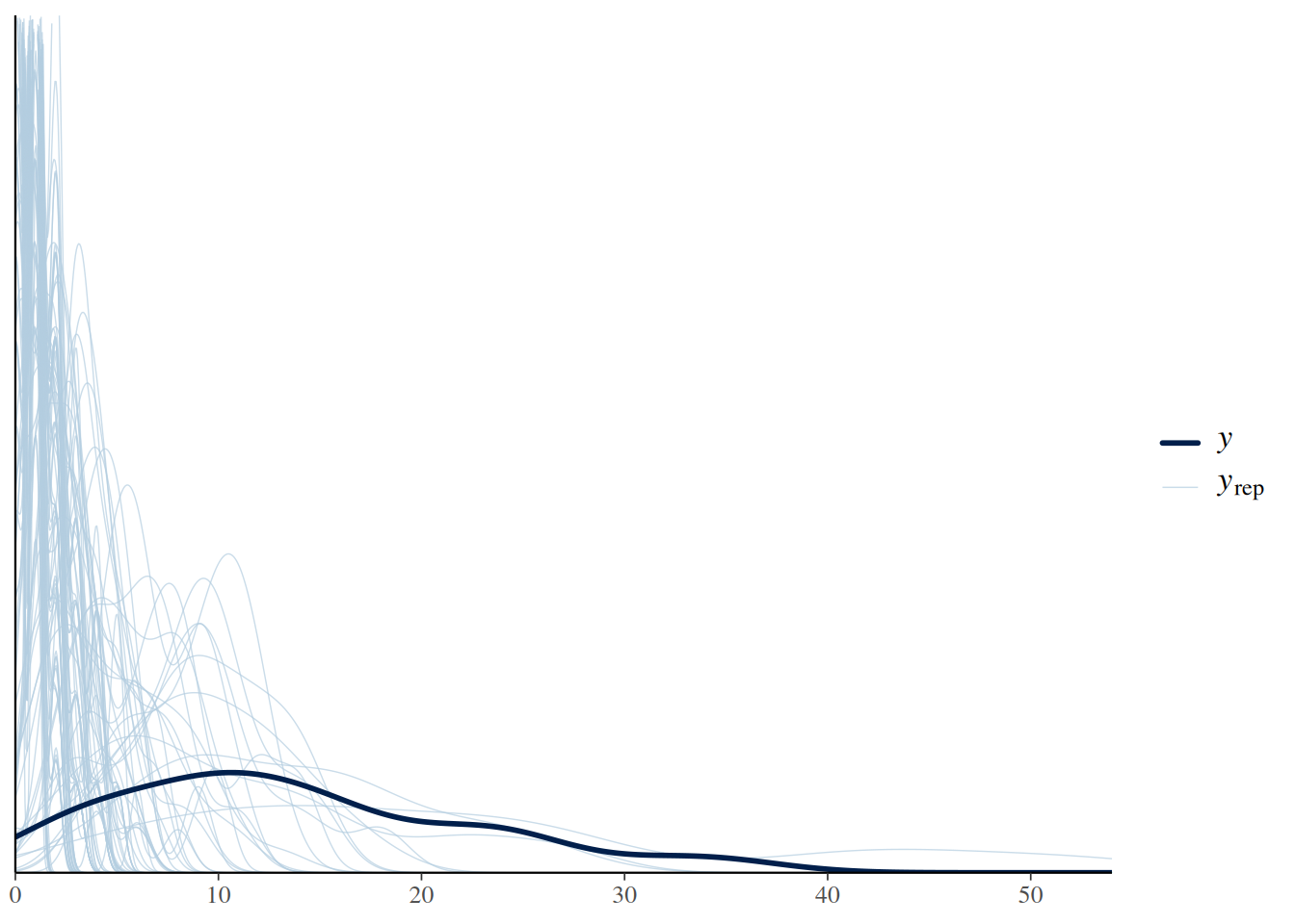
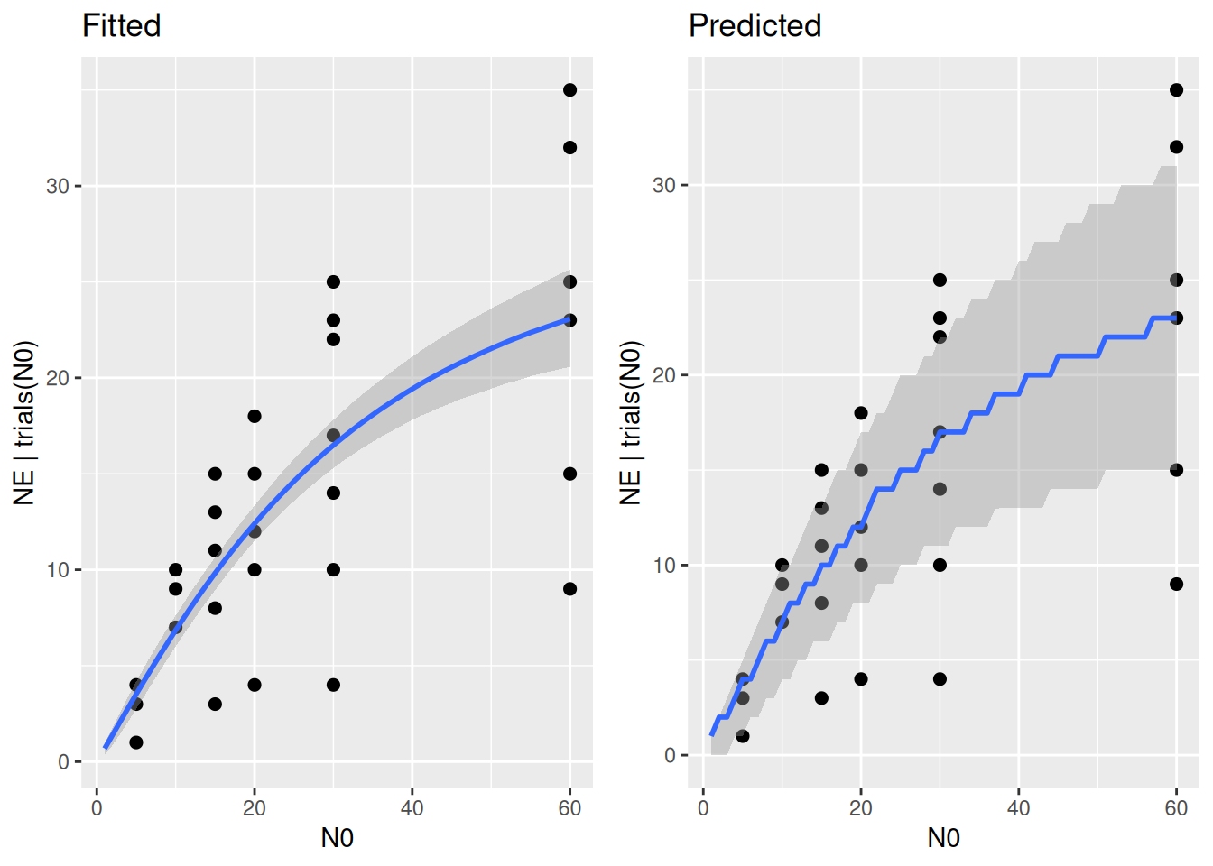
p1 = plot(conditional_effects(fit.1,
                              int_conditions = data.frame(N0=1:60)),
          points = TRUE, plot = FALSE)
p1 = p1[[1]] + ggtitle("Fitted")
p2 = plot(conditional_effects(fit.1,
                              int_conditions = data.frame(N0=1:60),
                              method = "posterior_predict" ),
          points = TRUE, plot = FALSE)
p2 = p2[[1]] + ggtitle("Predicted")
plot_grid(p1,p2)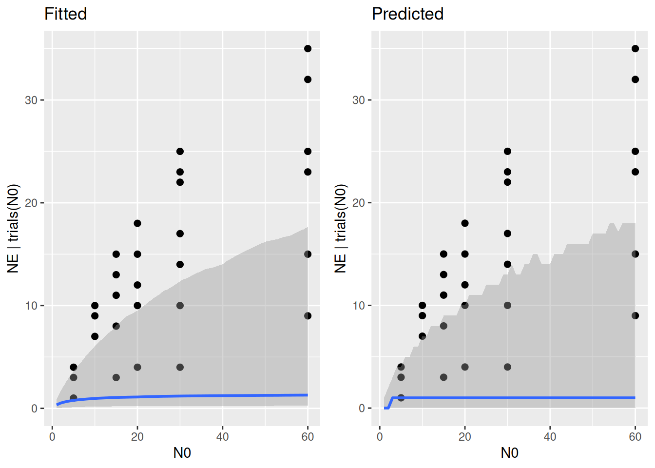
Here, predictions are biased towards lower feeding rates. This is because maximum feeding rate is given by \(f_\max=1/h\), the inverse of handling time. Each prior sample for \(h>1\) creates an \(f_\max<1\), which is unrealistic here. Fitting the actual model to the data will pull the posterior for \(h\) to lower values (which are not ruled out by this prior either), but we can define a more realistic prior for \(h\).
Prior predictive check 2
Conveniently, both maximum feeding rate \(f_\max\) and also the exponential distribution’s rate parameter \(\lambda\) express the inverse of handling time \(1/h\), so we choose a prior which is more coherent with maximum feeding here:
FR.priors  = c(prior(exponential(1.0), nlpar="a", lb=0),
               prior(exponential(30.0), nlpar="h", lb=0)
)
fit.1 = brm(FR.formula,
            family   = binomial(link="identity"),
            prior    = FR.priors,
            data     = df,
            cores    = 4,
            stanvars = stanvar(scode=Type2H_dyn_code, block="functions"),
            sample_prior = "only"
)
expose_functions(fit.1, vectorize=TRUE)pp_check(fit.1, ndraws=100)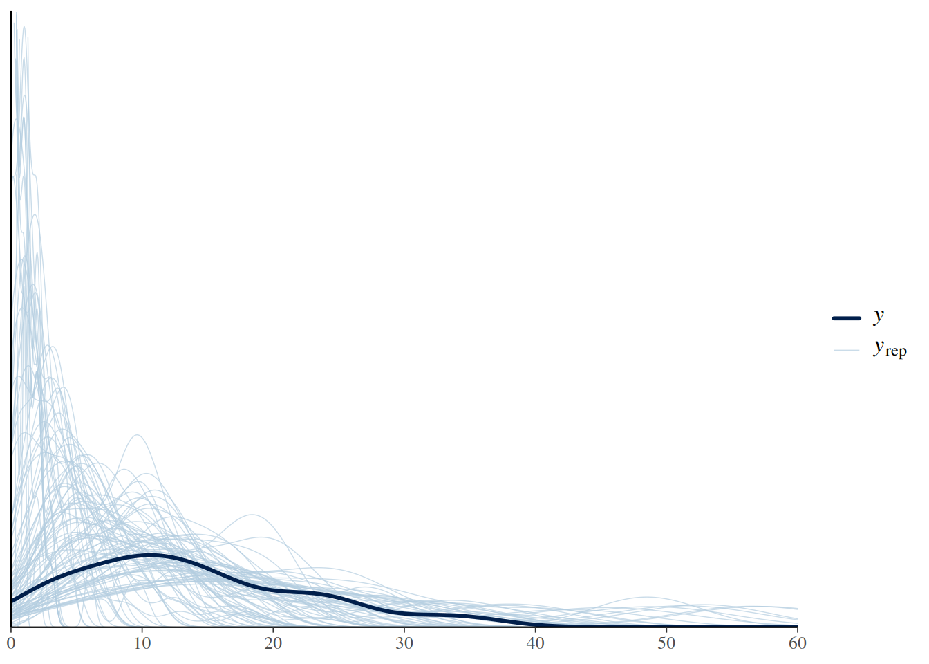
p1 = plot(conditional_effects(fit.1,
                              int_conditions = data.frame(N0=1:60)),
          points = TRUE, plot = FALSE)
p1 = p1[[1]] + ggtitle("Fitted")
p2 = plot(conditional_effects(fit.1,
                              int_conditions = data.frame(N0=1:60),
                              method = "posterior_predict" ),
          points = TRUE, plot = FALSE)
p2 = p2[[1]] + ggtitle("Predicted")
plot_grid(p1,p2)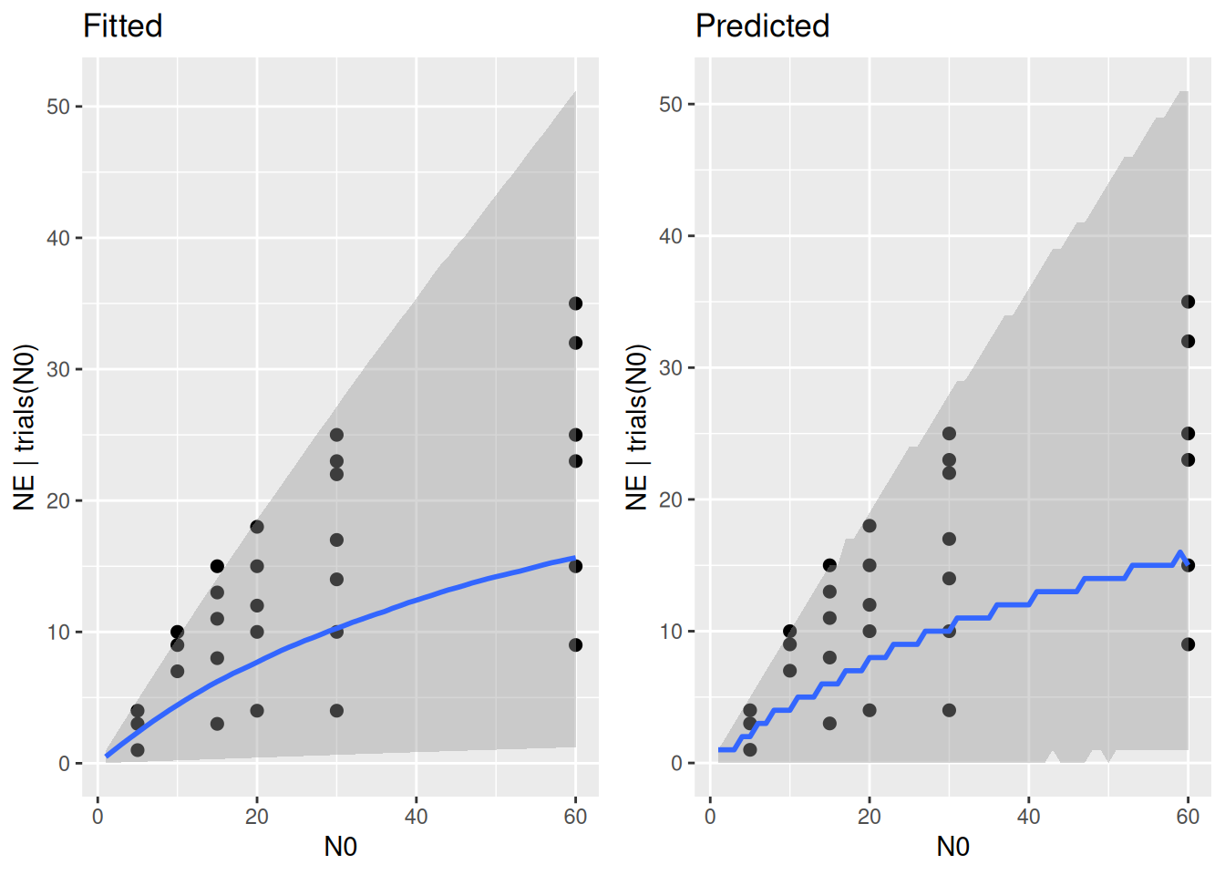
Now we see predictions widely covering all data (note that the upper limit of predictions is given by the 1-1 line \(N_E=N_0\)). Here, the prior does not make particularly biased predictions (prior too narrow), and also does not make completely unrealistic predictions (prior too wide). This is what we should ideally aim for, and we move on fitting the model to the data.
Model fit
fit.1 = brm(FR.formula,
            family   = binomial(link="identity"),
            prior    = FR.priors,
            data     = df,
            cores    = 4,
            stanvars = stanvar(scode=Type2H_dyn_code, block="functions")
)
summary(fit.1)
Family: binomial
Links: mu = identity
Formula: NE | trials(N0) ~ Type2H_dyn(N0, 1, 1, a, h)/N0
a ~ 1
h ~ 1
Data: df (Number of observations: 29)
Draws: 4 chains, each with iter = 2000; warmup = 1000; thin = 1;
total post-warmup draws = 4000
Regression Coefficients:
Estimate Est.Error l-95% CI u-95% CI Rhat Bulk_ESS Tail_ESS
a_Intercept 1.50 0.21 1.12 1.96 1.00 1252 1550
h_Intercept 0.03 0.00 0.02 0.04 1.00 1247 1481
Draws were sampled using sampling(NUTS). For each parameter, Bulk_ESS
and Tail_ESS are effective sample size measures, and Rhat is the potential
scale reduction factor on split chains (at convergence, Rhat = 1).Now that we have the actual posterior distribution, we plot it against the priors (drawing exponential density function as a curve).
p1 = mcmc_dens(fit.1, pars=c("b_a_Intercept")) +
  geom_function(fun=dexp, args=list(1.0), colour="lightblue3", linewidth=1.5) +
  scale_x_continuous(limits = c(0, 3))
p2 = mcmc_dens(fit.1, pars=c("b_h_Intercept")) +
  geom_function(fun=dexp, args=list(30.0), colour="lightblue3", linewidth=1.5) +
  scale_x_continuous(limits = c(0, 0.1))
plot_grid(p1, p2)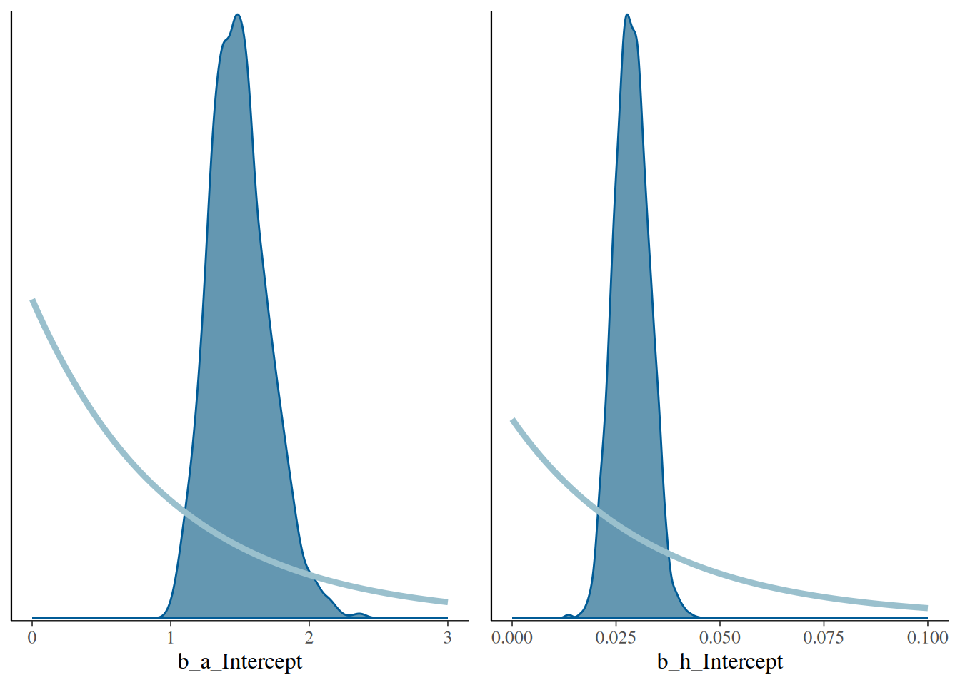
p1 = plot(conditional_effects(fit.1,
                              int_conditions = data.frame(N0=1:60)),
          points = TRUE, plot = FALSE)
p1 = p1[[1]] + ggtitle("Fitted")
p2 = plot(conditional_effects(fit.1,
                              int_conditions = data.frame(N0=1:60),
                              method = "posterior_predict" ),
          points = TRUE, plot = FALSE)
p2 = p2[[1]] + ggtitle("Predicted")
plot_grid(p1,p2)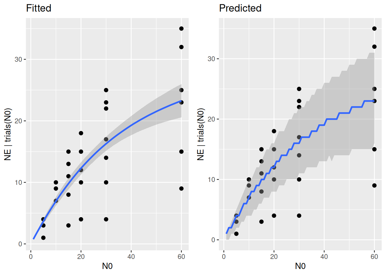
Strong priors: gamma distribution
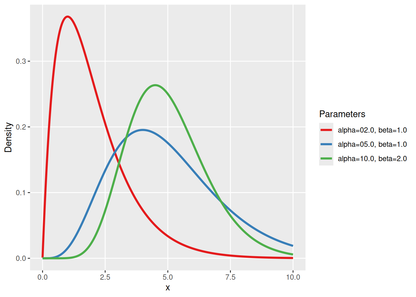
The exponential distribution works fine for vague priors, but it comes with 2 disadvantages if we want to use informative priors: First, it always allows values close to 0 and second, the variance is given by the mean. The gamma distribution is a strictly positive distribution as well, but it allows more flexibility via 2 parameters: shape \(\alpha\) and rate \(\beta\). It has a mean of \(\alpha/\beta\) and a variance of \(\alpha/\beta^2\). For instance, \(\alpha=5,\beta=1\) has mean 5, and so has every gamma distribution with \(\alpha=c\cdot 5,\beta=c\cdot 1\), but increasing \(c\) will decrease the variance.
The inverse gamma distribution for a parameter \(\theta\) is a distribution, whose inverse \(1/\theta\) has a gamma distribution with shape \(\alpha\) and rate \(\beta\). We use it as a prior distribution for \(h\), parameterized on the scale of \(f_\max=1/h\) (\(f_\max\) has a gamma prior).
Prior predictive check 1
Let’s say we have some prior information on attack rates being around \(a=2\) and maximum feeding rate being around \(f_\max=30\), i.e. \(h=1/30\). We choose gamma distributions with rate parameters \(\beta=1\), respectively, and perform prior predictive checks.
FR.formula = bf( NE | trials(N0) ~ Type2H_dyn(N0,1.0,1.0,a,h)/N0,
                 a~1, h~1,
                 nl = TRUE)
FR.priors  = c(prior(gamma(2.0, 1.0), nlpar="a", lb=0),
               prior(inv_gamma(30.0, 1.0), nlpar="h", lb=0)
)
fit.2 = brm(FR.formula,
            family   = binomial(link="identity"),
            prior    = FR.priors,
            data     = df,
            cores    = 4,
            stanvars = stanvar(scode=Type2H_dyn_code, block="functions"),
            sample_prior = "only"
)
expose_functions(fit.2, vectorize=TRUE)pp_check(fit.2, ndraws=100)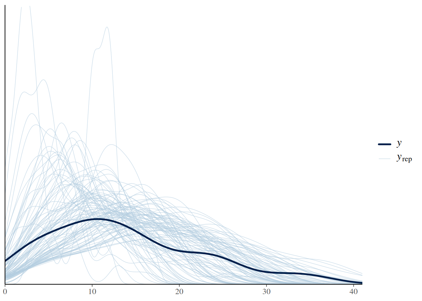
p1 = plot(conditional_effects(fit.2,
                              int_conditions = data.frame(N0=1:60)),
          points = TRUE, plot = FALSE)
p1 = p1[[1]] + ggtitle("Fitted")
p2 = plot(conditional_effects(fit.2,
                              int_conditions = data.frame(N0=1:60),
                              method = "posterior_predict" ),
          points = TRUE, plot = FALSE)
p2 = p2[[1]] + ggtitle("Predicted")
plot_grid(p1,p2)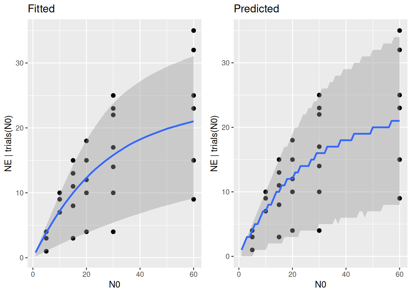
These priors still cover a wide range of the data’s variation. If this is the level of prior information we’d want to use that would be totally fine.
Prior predictive check 2
However, if we are more certain about the parameters’ means \(a=2\) and \(h=1/30\), we can decrease the priors’ variances by multiplying the shape and rate parameters by the same factor, here by factor 2.
FR.priors  = c(prior(gamma(2*2.0, 2*1.0), nlpar="a", lb=0),
               prior(inv_gamma(2*30.0, 2*1.0), nlpar="h", lb=0)
)
fit.2 = brm(FR.formula,
            family   = binomial(link="identity"),
            prior    = FR.priors,
            data     = df,
            cores    = 4,
            stanvars = stanvar(scode=Type2H_dyn_code, block="functions"),
            sample_prior = "only"
)
expose_functions(fit.2, vectorize=TRUE)pp_check(fit.2, ndraws=100)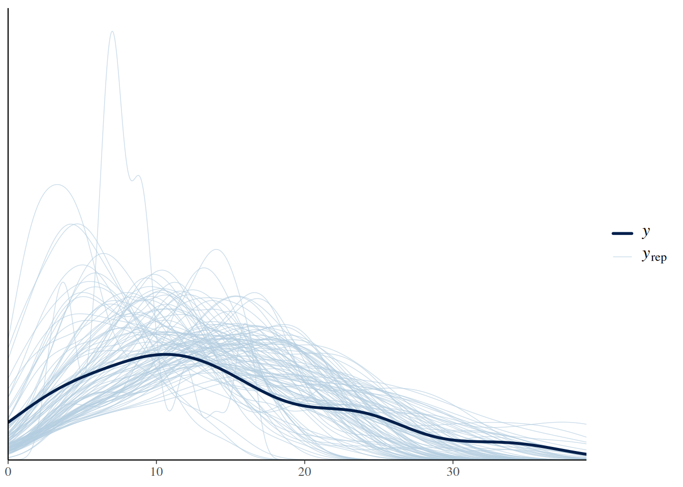
p1 = plot(conditional_effects(fit.2,
                              int_conditions = data.frame(N0=1:60)),
          points = TRUE, plot = FALSE)
p1 = p1[[1]] + ggtitle("Fitted")
p2 = plot(conditional_effects(fit.2,
                              int_conditions = data.frame(N0=1:60),
                              method = "posterior_predict" ),
          points = TRUE, plot = FALSE)
p2 = p2[[1]] + ggtitle("Predicted")
plot_grid(p1,p2)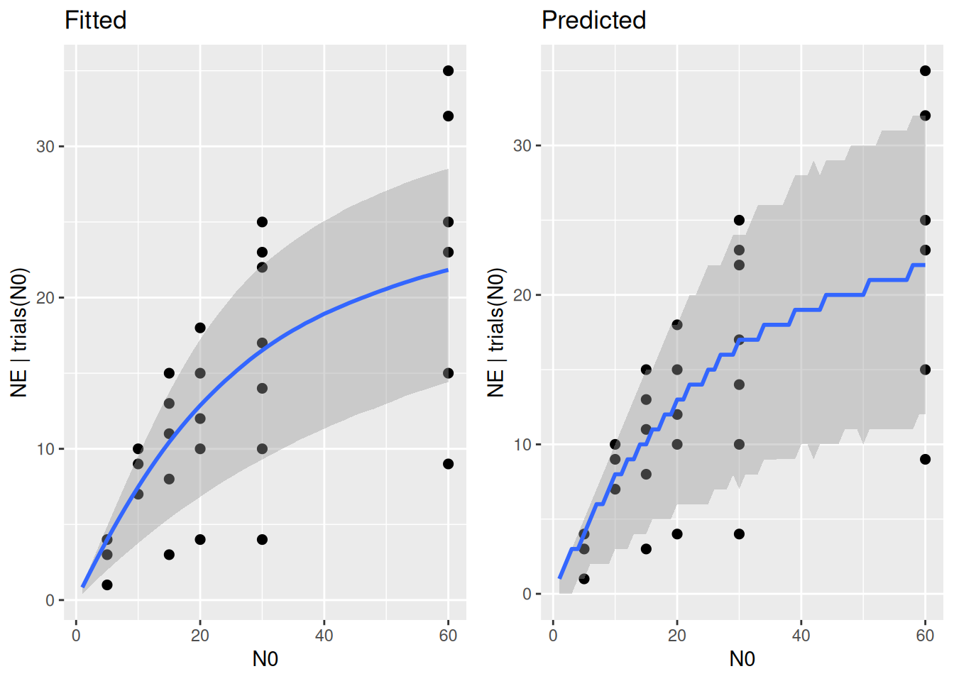
Model fit
The last prior choice is used for model fitting.
fit.2 = brm(FR.formula,
            family   = binomial(link="identity"),
            prior    = FR.priors,
            data     = df,
            cores    = 4,
            stanvars = stanvar(scode=Type2H_dyn_code, block="functions")
)
summary(fit.2)
Family: binomial
Links: mu = identity
Formula: NE | trials(N0) ~ Type2H_dyn(N0, 1, 1, a, h)/N0
a ~ 1
h ~ 1
Data: df (Number of observations: 29)
Draws: 4 chains, each with iter = 2000; warmup = 1000; thin = 1;
total post-warmup draws = 4000
Regression Coefficients:
Estimate Est.Error l-95% CI u-95% CI Rhat Bulk_ESS Tail_ESS
a_Intercept 1.64 0.19 1.31 2.05 1.00 1636 2019
h_Intercept 0.03 0.00 0.03 0.04 1.00 1664 2171
Draws were sampled using sampling(NUTS). For each parameter, Bulk_ESS
and Tail_ESS are effective sample size measures, and Rhat is the potential
scale reduction factor on split chains (at convergence, Rhat = 1).p1 = mcmc_dens(fit.2, pars=c("b_a_Intercept")) +
geom_function(fun=dgamma, args=list(2*2.0, 2*1.0), colour="lightblue3", linewidth=1.5) +
scale_x_continuous(limits = c(0, 3))
p2 = mcmc_dens(fit.2, pars=c("b_h_Intercept")) +
geom_function(fun=dinvgamma, args=list(2*30.0, 2*1.0), colour="lightblue3", linewidth=1.5) +
scale_x_continuous(limits = c(0, 0.1))
plot_grid(p1, p2)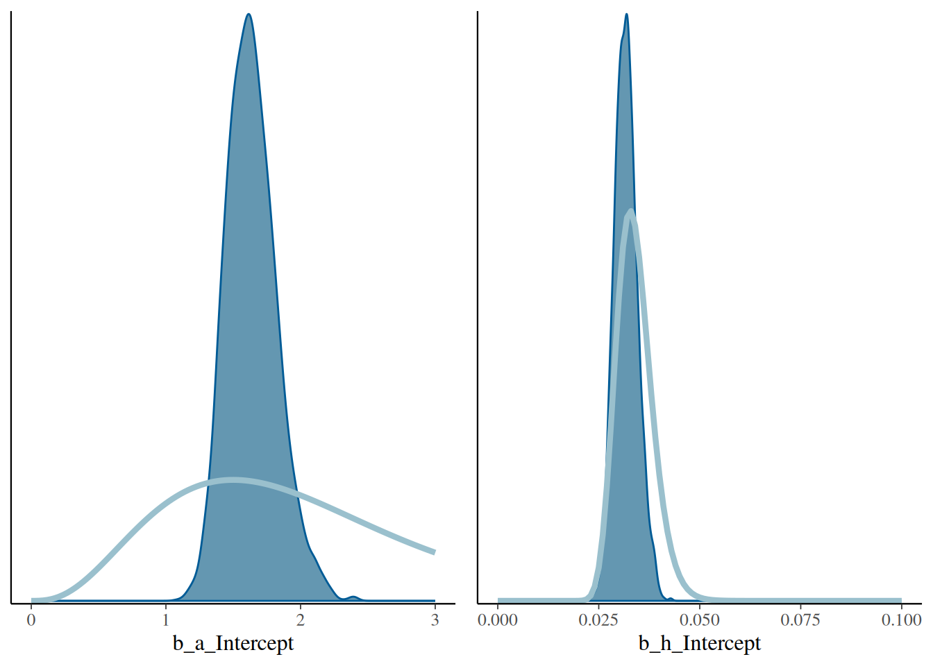
Plotting prior vs. posterior reveals that the prior was already quite informative on parameter \(h\) (posterior overlaps with the prior for the most part), but not so much on parameter \(a\) (prior much wider than posterior)
p1 = plot(conditional_effects(fit.2,
                              int_conditions = data.frame(N0=1:60)),
          points = TRUE, plot = FALSE)
p1 = p1[[1]] + ggtitle("Fitted")
p2 = plot(conditional_effects(fit.2,
                              int_conditions = data.frame(N0=1:60),
                              method = "posterior_predict" ),
          points = TRUE, plot = FALSE)
p2 = p2[[1]] + ggtitle("Predicted")
plot_grid(p1,p2)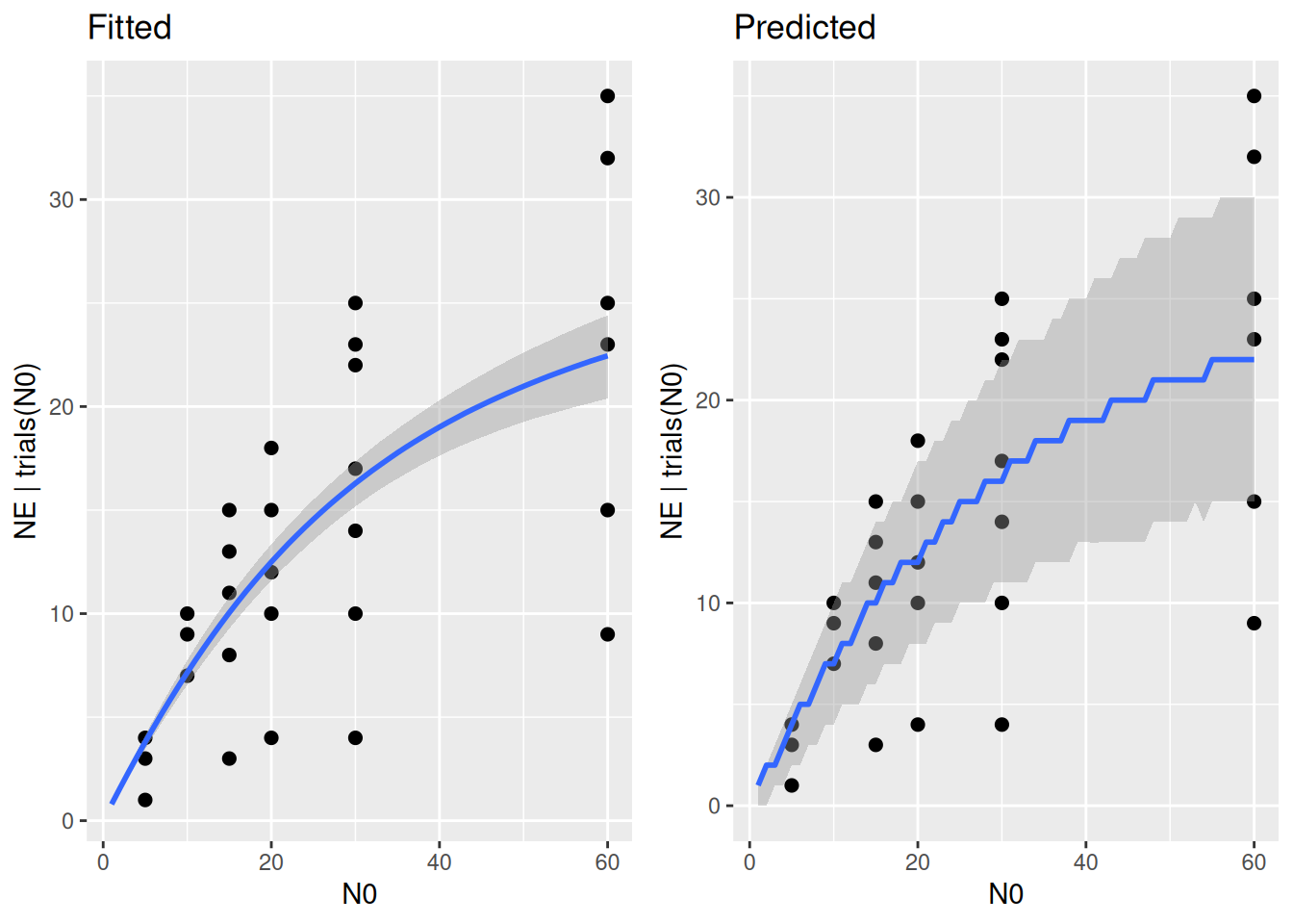
Reparameterization with f_max and N_half
The type 2 functional response can be rewritten as \[F(N)=\frac{f_\max N}{N_\text{half}+N}\] Here, parameters define maximum feeding rate \(f_\max\) and half-saturation density \(N_\text{half}\), which is the prey density where realized feeding rate is half of the maximum \(f_\max/2\). The original type 2 formulation \(F(N)=\frac{a N}{1+ahN}\) can be recovered using \(h=1/f_\max\) and \(a=f_\max/N_\text{half}\).
This reparameterization can make it easier to define priors, especially for the (generalized) type 3 functional response. This one reads \[F(N)=\frac{f_\max N^{1+q}}{N_\text{half}^{1+q}+N^{1+q}}\]
where \(f_\max\) and \(N_\text{half}\) have the same interpretation as above. The original type 3 formulation \(F(N)=\frac{b N^{1+q}}{1+bhN^{1+q}}\) is given for \(h=1/f_\max\) and \(b=f_\max/N_\text{half}^{1+q}\). It can be difficult to come up with meaningful priors for attack coefficient \(b\), and it is most likely not independent of \(q\) (both define attack rate \(a=bN^{1+q}\)). \(N_\text{half}\), however, is independent of \(q\) and priors for \(f_\max\), \(N_\text{half}\) and \(q\) can be specified independently.
The reparameterization is defined via nlf() in the model formula, and works analogously for the type 2 and the strict type 3 (with fixed exponent \(q=1\)).
FR.formula = bf( NE | trials(N0) ~ Type3GenH_dyn(N0,1.0,1.0,b,h,q)/N0,
                 nlf(b ~ fmax/Nhalf^(1.0+q)),
                 nlf(h ~ 1.0/fmax),
                 fmax + Nhalf + q ~ 1,
                 nl = TRUE)
Prior predictive check
We here define normal distributions for all parameters, but specify appropriate lower boundaries. They have relatively wide standard deviations and are intended as weakly informative priors.
FR.priors  = c(prior(normal(30, 15), nlpar="fmax", lb=1),
               prior(normal(20, 10), nlpar="Nhalf", lb=1),
               prior(normal(0,1), nlpar="q", lb=-1.0)
)
fit.3 = brm(FR.formula,
            family   = binomial(link="identity"),
            prior    = FR.priors,
            data     = df,
            cores    = 4,
            stanvars = stanvar(scode=Type3GenH_dyn_code, block="functions"),
            sample_prior = "only"
)
expose_functions(fit.3, vectorize=TRUE)pp_check(fit.3, ndraws=100) 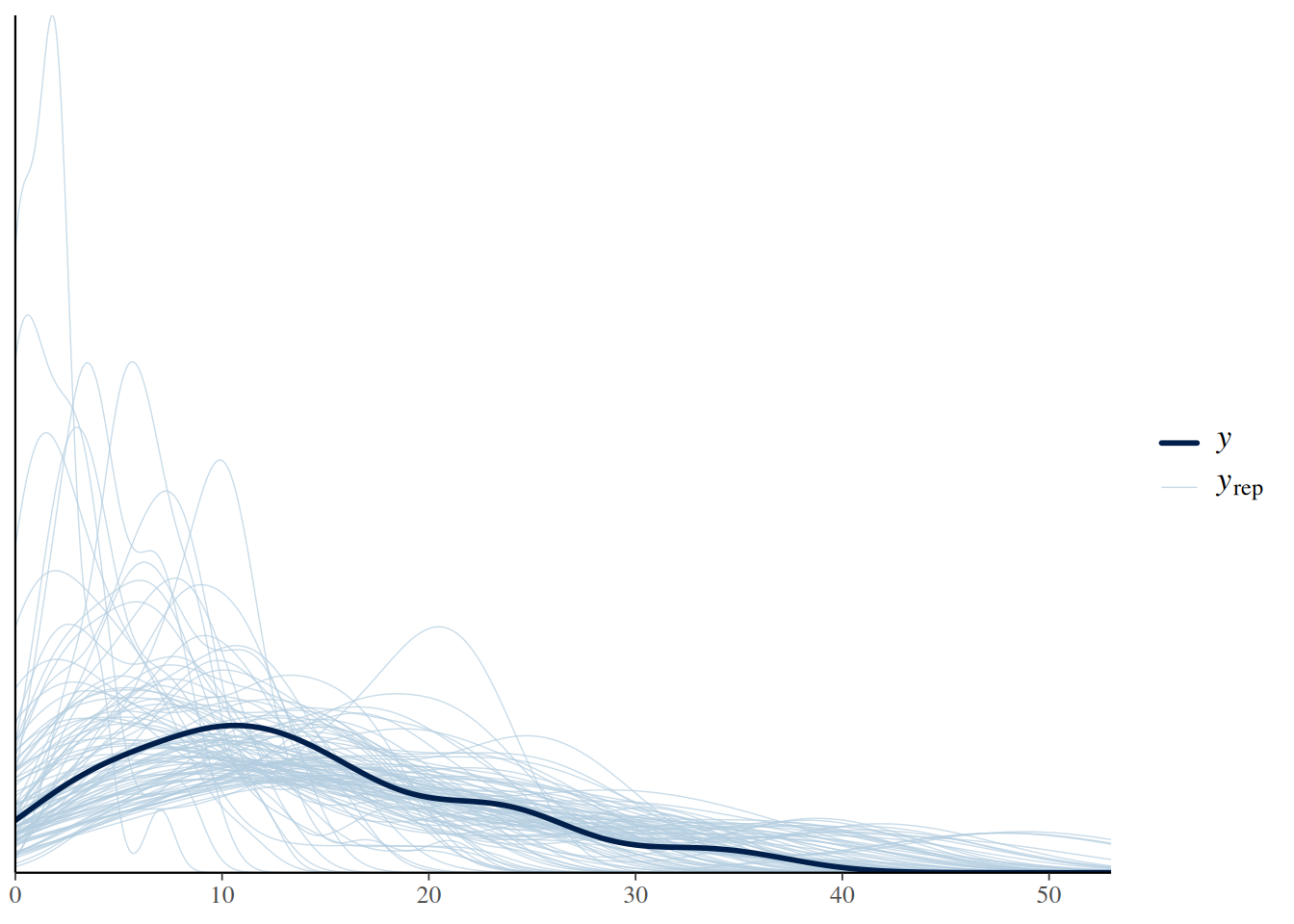
p1 = plot(conditional_effects(fit.3,
                              int_conditions = data.frame(N0=1:60)),
          points = TRUE, plot = FALSE)
p1 = p1[[1]] + ggtitle("Fitted")
p2 = plot(conditional_effects(fit.3,
                              int_conditions = data.frame(N0=1:60),
                              method = "posterior_predict" ),
          points = TRUE, plot = FALSE)
p2 = p2[[1]] + ggtitle("Predicted")
plot_grid(p1,p2)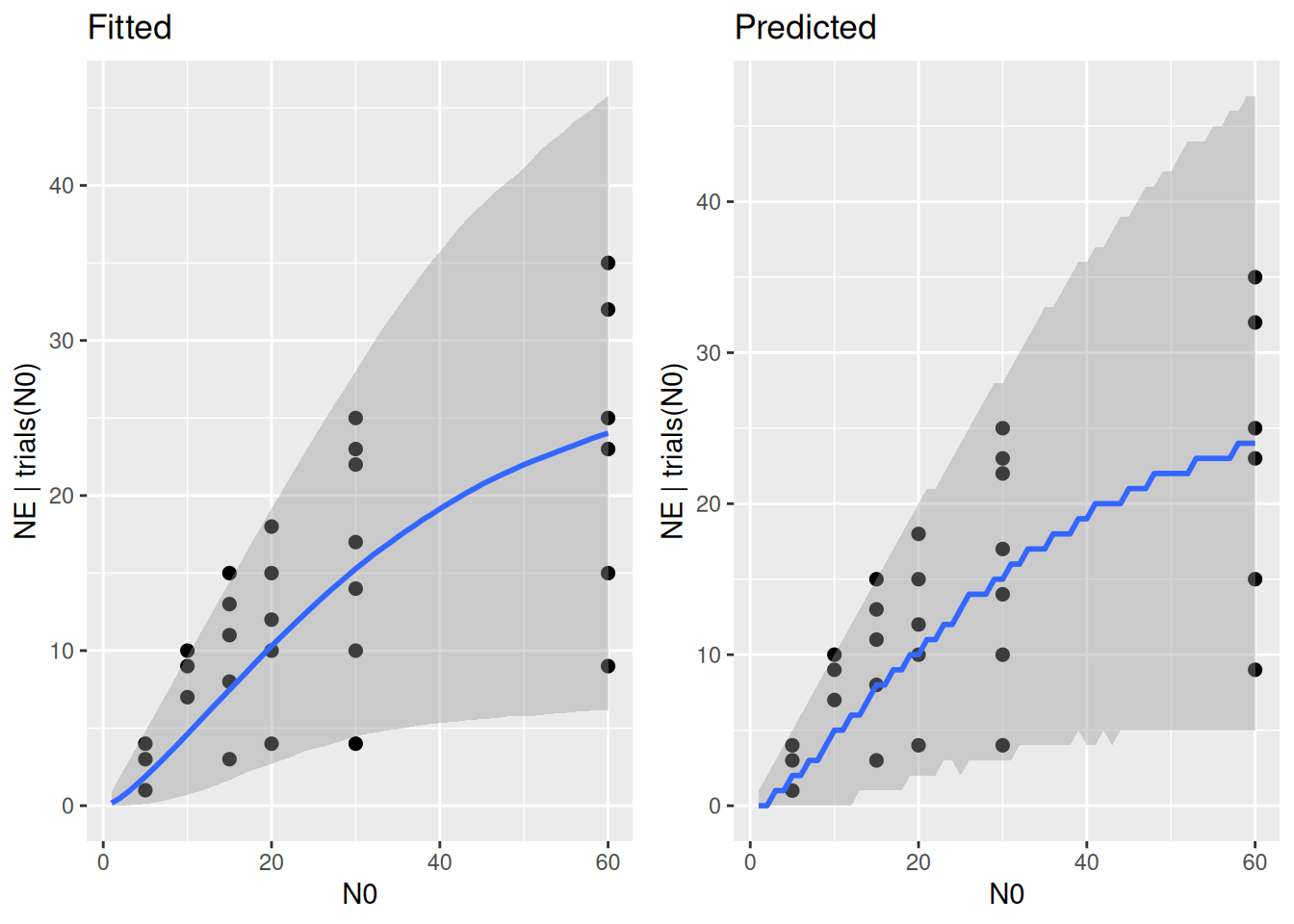
Posterior predictive checks and coverage of observations are adequate for weakly informative priors, and we fit the model next.
Model fit
fit.3 = brm(FR.formula,
            family   = binomial(link="identity"),
            prior    = FR.priors,
            data     = df,
            cores    = 4,
            stanvars = stanvar(scode=Type3GenH_dyn_code, block="functions")
)
summary(fit.3)
Family: binomial
Links: mu = identity
Formula: NE | trials(N0) ~ Type3GenH_dyn(N0, 1, 1, b, h, q)/N0
b ~ fmax/Nhalf^(1 + q)
h ~ 1/fmax
fmax ~ 1
Nhalf ~ 1
q ~ 1
Data: df (Number of observations: 29)
Draws: 4 chains, each with iter = 2000; warmup = 1000; thin = 1;
total post-warmup draws = 4000
Regression Coefficients:
Estimate Est.Error l-95% CI u-95% CI Rhat Bulk_ESS Tail_ESS
fmax_Intercept 32.43 4.94 23.64 42.71 1.01 918 1107
Nhalf_Intercept 20.63 6.38 10.79 35.41 1.01 926 1036
q_Intercept 0.12 0.19 -0.16 0.56 1.01 988 1230
Draws were sampled using sampling(NUTS). For each parameter, Bulk_ESS
and Tail_ESS are effective sample size measures, and Rhat is the potential
scale reduction factor on split chains (at convergence, Rhat = 1).The summary table displays model parameters only, but summaries for \(b\) and \(h\) (as functions of model parameters) are computed with fitted()
fitted(fit.3, nlpar="b", newdata=data.frame(N0=1)) Estimate Est.Error Q2.5 Q97.5
[1,] 1.289347 0.4659735 0.4730732 2.271127fitted(fit.3, nlpar="h", newdata=data.frame(N0=1)) Estimate Est.Error Q2.5 Q97.5
[1,] 0.03156796 0.004883592 0.02341485 0.04229833Plotting prior vs. posterior:
p1 = mcmc_dens(fit.3, pars=c("b_fmax_Intercept")) +
  geom_function(fun=dnorm, args=list(30, 15), colour="lightblue3", linewidth=1.5) +
  scale_x_continuous(limits = c(0, 50))
p2 = mcmc_dens(fit.3, pars=c("b_Nhalf_Intercept")) +
  geom_function(fun=dnorm, args=list(20, 10), colour="lightblue3", linewidth=1.5) +
  scale_x_continuous(limits = c(0, 50))
p3 = mcmc_dens(fit.3, pars=c("b_q_Intercept")) +
  geom_function(fun=dnorm, args=list(0, 1), colour="lightblue3", linewidth=1.5) +
  scale_x_continuous(limits = c(-0.5, 1.0))
plot_grid(p1, p2, p3, ncol=3)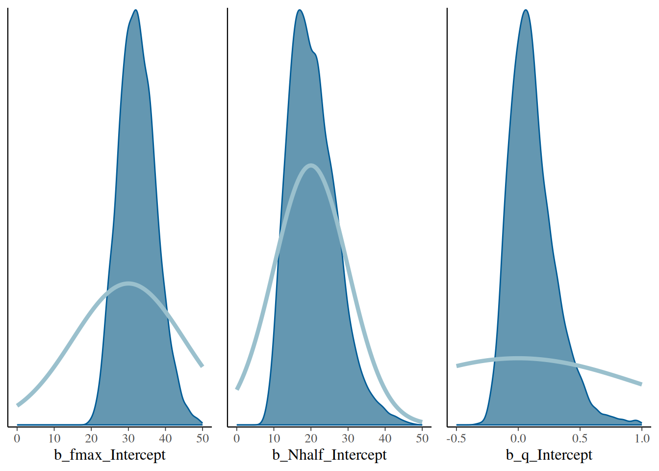
p1 = plot(conditional_effects(fit.3,
                              int_conditions = data.frame(N0=1:60)),
          points = TRUE, plot = FALSE)
p1 = p1[[1]] + ggtitle("Fitted")
p2 = plot(conditional_effects(fit.3,
                              int_conditions = data.frame(N0=1:60),
                              method = "posterior_predict" ),
          points = TRUE, plot = FALSE)
p2 = p2[[1]] + ggtitle("Predicted")
plot_grid(p1,p2)