rm(list=ls())
library(BayesFR)
library(brms)
library(ggplot2)2. Minimal example: data without prey replacement
This dataset is originally from Hossie and Murray (2010) and was made available in the FoRAGE database (Uiterwaal et al. 2022). It includes data for a dragonfly nymph predator feeding on tadpoles in three leaf litter treatments. Here, we will regress number of eaten prey \(N_E\) against initial prey abundance \(N_0\). All experiments were run for 24 hours and eaten prey were not replaced. We are using the high leaf litter treatment.
data(df_Hossie_and_Murray_2010_OECOLOGIA)
df = subset(df_Hossie_and_Murray_2010_OECOLOGIA, ID=="Figure 1e")
head(df)
N0 NE Time Predator Prey ID
63 5 1 24 Anax junius Rana pipiens Figure 1e
64 5 3 24 Anax junius Rana pipiens Figure 1e
65 5 4 24 Anax junius Rana pipiens Figure 1e
66 10 7 24 Anax junius Rana pipiens Figure 1e
67 10 9 24 Anax junius Rana pipiens Figure 1e
68 10 10 24 Anax junius Rana pipiens Figure 1eggplot(aes(N0,NE), data=df) +
geom_jitter(width=0.1, height=0.0, alpha=0.6, size=2.5) +
coord_cartesian(xlim=c(0,NA), ylim=c(0,NA))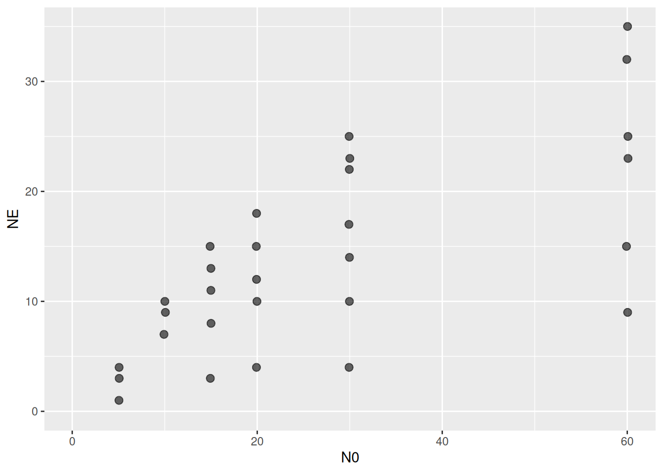
We intend to estimate a type 3 functional response, which has a density-dependent attack rate \(a=bN\), and is parameterized with attack rate coeffient \(b\) and handling time \(h\). Since eaten prey were not replaced (and number of available prey is not constant), we cannot directly fit the type 3 functional response \[ F(N) = \frac{bN^2}{1+bhN^2}PT\] to the observed data. Instead, prey abundance is modeled dynamically by the differential equation \[ \frac{dN}{dt} = -\frac{bN^2}{1+bhN^2}P, \quad N(t=0)=N_0\] With its solution in the interval \(t=[0,T]\), the final number of prey \(N(t=T)=N_T\) is used to compute predictions \(\hat{N}_E=N_0-N_T\). Analytical solutions exist for the type 2 FR (LambertW formula) and the type 3 FR (quadratic equation), which are used in this package. For other functional responses, such as the generalized type 3 FR with a flexible exponent \(q\), a numerical solution of the corresponding differential equation is implemented. An alternative parameterization \(\frac{f_\max N^2}{N_\text{half}^2+N^2}\) using maximum feeding rate and half-saturation density is presented in the priors tutorial.
Then, we still need to define a likelihood function for model fitting. Observed numbers of eaten prey are integers bounded between \(0\) and \(N_0\), because the predator cannot eat more than the initial abundance. This makes the Binomial distribution \[N_E\sim\text{Binomial}\left(n,\ p\right)\] with \(n=N_0\) trials and individual prey probability of being eaten \(p=\frac{N_0-N_T}{N_0}\) an obvious choice. Alternatively, the Beta Binomial distribution for overdispersed data is discussed in the tutorial on likelihood functions.
The dynamical prediction model is defined by the function Type3H_dyn() and coded in Type3H_dyn_code (which is used later in the brms call). It computes number of eaten prey based on these arguments: abundance of offered prey N0, predator abundance P0, experimental duration Time, and parameters b and h, in that exact order. We define the brms formula:
FR.formula = bf( NE | trials(N0) ~ Type3H_dyn(N0,1.0,1.0,b,h)/N0,
                 b~1, h~1,
                 nl = TRUE)
For the Binomial distribution, the number of trials N0 is specified, and the success probability must be computed by dividing predicted number of eaten Type3H_dyn() by number of trials N0. Here, we provided fixed values for P0=1.0 and Time=1.0 [day], which means parameters are also estimated in [day].
As in the previous example, we choose some very weakly informative priors, the lower boundary lb=0 is required to keep parameters non-negative.
FR.priors  = c(prior(exponential(1.0), nlpar="b", lb=0),
               prior(exponential(1.0), nlpar="h", lb=0))
We fit the model calling brm() with the model formula. The Binomial distribution is specified in family with the identity link, overwriting the default logit link (which is not required here because success probabilities are already bounded between 0 and 1). stanvars contains this package’s code for the prediction model Type3H_dyn_code. After the model is run, this function is made available to R via expose_functions(), which is required for computing model predictions.
fit.1 = brm(FR.formula,
            family   = binomial(link="identity"),
            prior    = FR.priors,
            data     = df,
            cores    = 4,
            stanvars = stanvar(scode=Type3H_dyn_code, block="functions")
)
expose_functions(fit.1, vectorize=TRUE)
We check the summary table and the traceplots for MCMC convergence (Rhat values <1.01 and good mixing of the chains):
summary(fit.1) Family: binomial
Links: mu = identity
Formula: NE | trials(N0) ~ Type3H_dyn(N0, 1, 1, b, h)/N0
b ~ 1
h ~ 1
Data: df (Number of observations: 29)
Draws: 4 chains, each with iter = 2000; warmup = 1000; thin = 1;
total post-warmup draws = 4000
Regression Coefficients:
Estimate Est.Error l-95% CI u-95% CI Rhat Bulk_ESS Tail_ESS
b_Intercept 0.26 0.06 0.17 0.40 1.00 1449 1996
h_Intercept 0.05 0.00 0.04 0.05 1.00 1409 1861
Draws were sampled using sampling(NUTS). For each parameter, Bulk_ESS
and Tail_ESS are effective sample size measures, and Rhat is the potential
scale reduction factor on split chains (at convergence, Rhat = 1).plot(fit.1)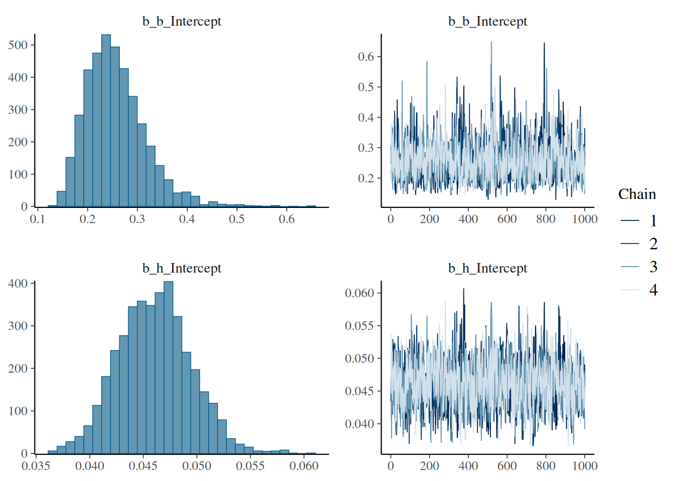
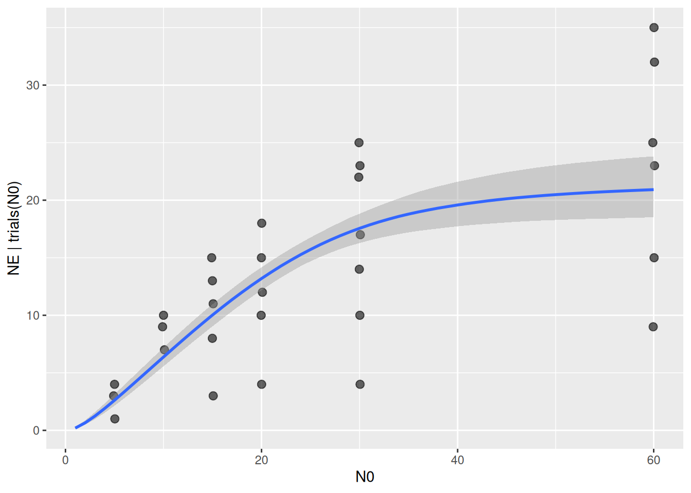
Finally, we plot model predictions against the observed data with conditional_effects(). This function uses samples from the parameters’ posterior distribution to compute posterior predictions of fitted values, which are displayed as mean fitted value (in blue) and 95% credible intervals (gray).
plot(conditional_effects(fit.1), points=TRUE)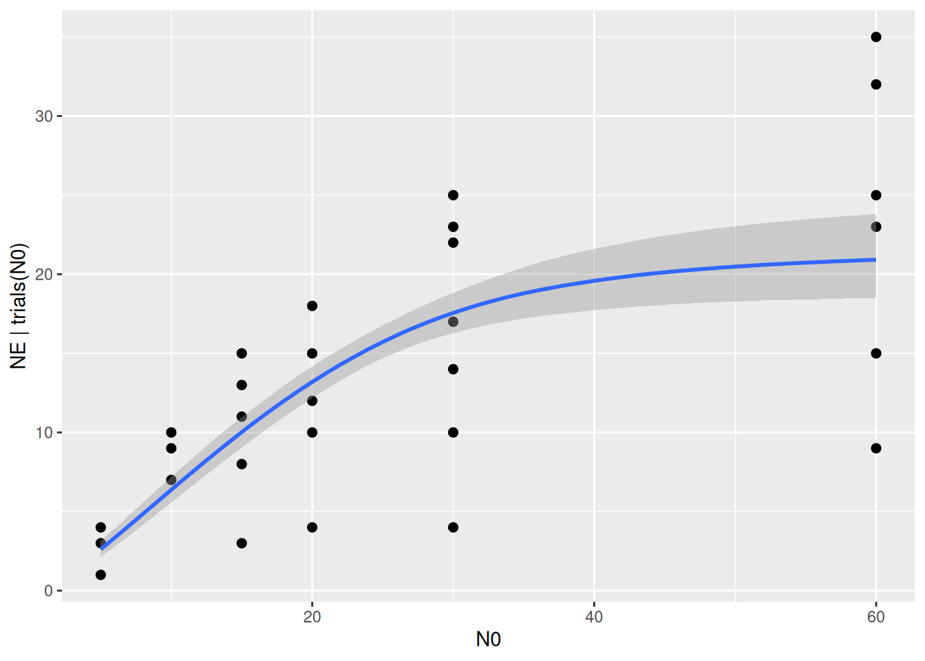
The plot can be modified to show the sigmoidal shape of the type 3 FR at low abundances. For a fully customizable plot, the output can also be saved in a ggplot object with p = conditional_effects().
plot(conditional_effects(fit.1,
                         effects="N0",
                         int_conditions=data.frame(N0=1:60)),
     points=TRUE, point_args=list(width=0.1, alpha=0.6, size=2.5))