Should you scale your time series for nonlinear analysis?

Population and community time series are often scaled (mean-centered and scaled by standard deviation) before analysis. While this works with linear models, it generally does not with nonlinear analysis. This also depends on whether you analyze on a linear or on log-scale.

Linear and nonlinear analysis

Linear time series analysis is popular with observed time series of community abundances from the field. Classically, a multivariate time series of \(n\) species \(X_t=(x_{1,t},\dots,x_{n,t})\) is log-transformed \(Y_t=\log(X_t)\), before a multivariate autoregressive model MAR(1) is fitted \[ y_{i,t+1}=y_{i,t} + a_i+\sum_{j=1}^n b_{ij}y_{j,t}+\sum_{j=1}^m c_{ij}u_{j,t} + \varepsilon_{i,t}, \] see e.g. Ives et al. (2003), Mutshinda, O’Hara & Woiwod (2009), Hampton et al. (2013). With matrix algebra, this can be written as \[ Y_{t+1}=Y_{t} + A+BY_{t}+CU_{t} + \varepsilon_{t} \] where \(B\) is an interaction matrix, and \(C\) contains the effects of environmental variables \(U_t\). This model is purely linear. The MARSS package is a popular tool for analysis (Holmes, Ward & Wills 2012).

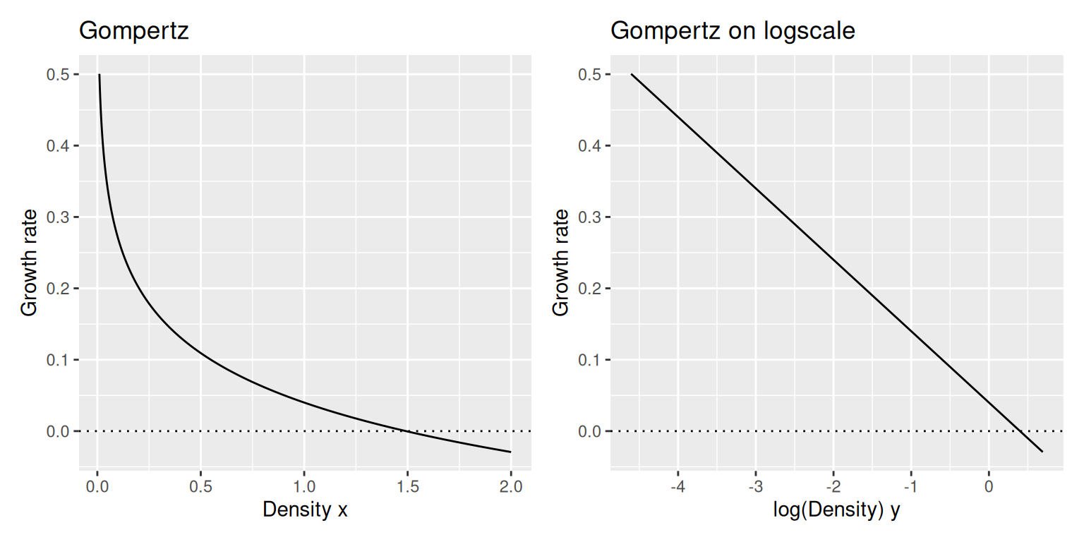
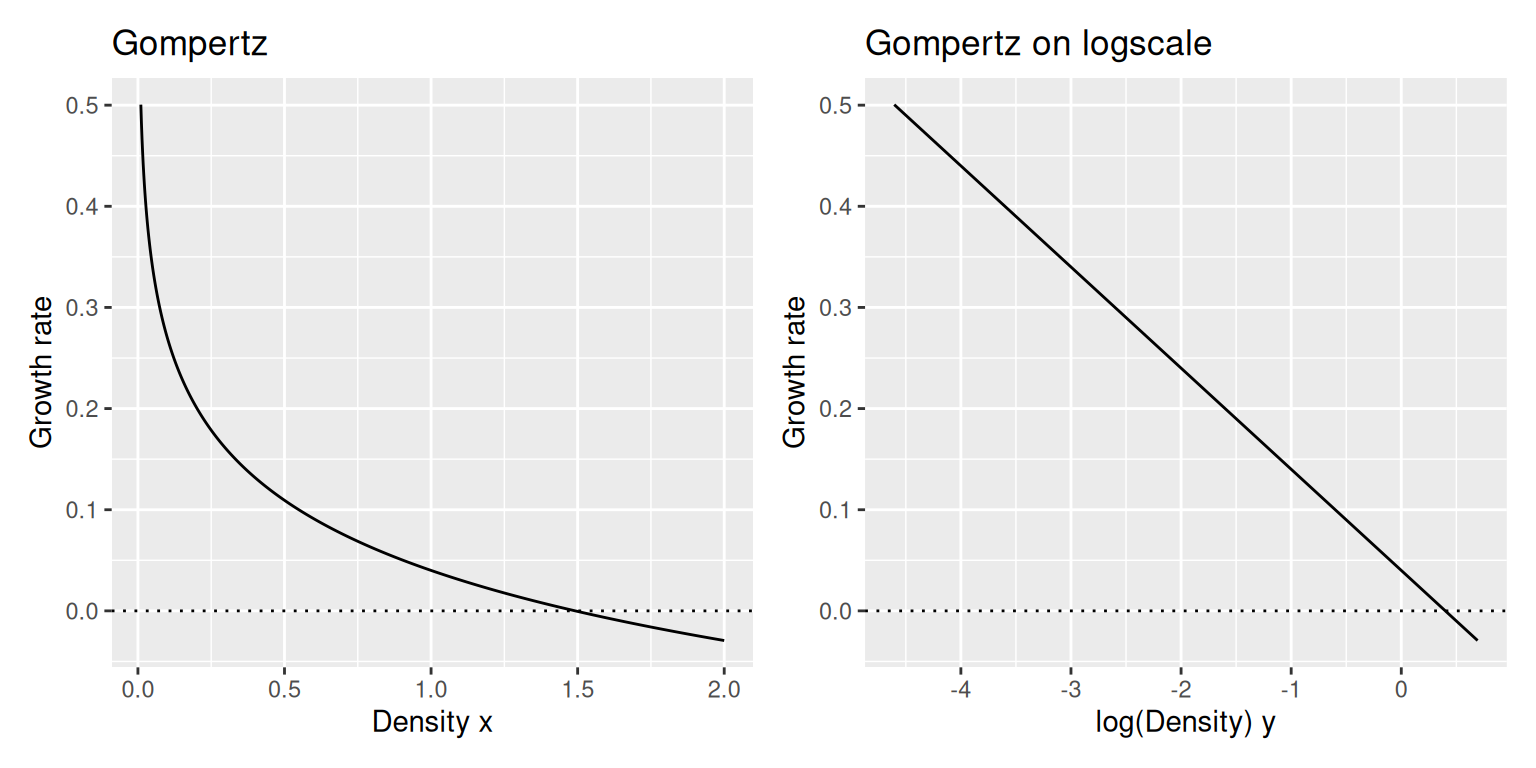
This MAR(1) model actually corresponds to an ecological community model. If we transform densities back to the original scale, we get the discrete-time, multi-species Gompertz model.
\[ \begin{align} x_{i,t+1} &= \exp(y_{i,t+1}) \\ &= \exp\left( y_{i,t} + a_i+\sum_{j=1}^n b_{ij}\textcolor{red}{y_{j,t}}+\sum_{j=1}^m c_{ij}u_{j,t} + \varepsilon_{i,t} \right) \\ &=x_{i,t} \cdot \exp\left( a_i+\sum_{j=1}^n b_{ij}\textcolor{red}{y_{j,t}}+\sum_{j=1}^m c_{ij}u_{j,t} + \varepsilon_{i,t} \right) \\ &=x_{i,t} \cdot \exp\left( a_i+\sum_{j=1}^n b_{ij}\textcolor{red}{\log(x_{j,t})}+\sum_{j=1}^m c_{ij}u_{j,t} + \varepsilon_{i,t} \right) \end{align} \]

More common in modeling, however, is the generalized Lotka-Volterra model. In its discrete-time version, the Ricker model, it reads \[ x_{i,t+1} =x_{i,t} \cdot \exp\left( a_i+\sum_{j=1}^n b_{ij}\textcolor{red}{x_{j,t}}+\sum_{j=1}^m c_{ij}u_{j,t} + \varepsilon_{i,t} \right), \] e.g. Mutshinda et al. (2023). On logscale, it becomes an additive model just like the Gompertz model, although it is no longer linear in \(y\). However, it is still linear in its parameters. I.e., under certain assumptions (observation error is negligible compared to process error) and by defining new predictors \(\exp(y_i)\), it can be pushed through MARSS or even lm(...) to estimate all parameters [seperate blog post coming soon]. \[ \begin{align} y_{i,t+1} &=y_{i,t} + a_i+\sum_{j=1}^n b_{ij}\textcolor{red}{x_{j,t}}+\sum_{j=1}^m c_{ij}u_{j,t} + \varepsilon_{i,t} \\ &=y_{i,t} + a_i+\sum_{j=1}^n b_{ij}\textcolor{red}{\exp(y_{j,t})}+\sum_{j=1}^m c_{ij}u_{j,t} + \varepsilon_{i,t} \\ \end{align} \]

Scaling and reparametrization

For the linear MAR(1) / Gompertz model, it makes sense to scale log-transformed observations \(y_{i,t}\) species-wise, i.e., \(\tilde y_{i,t}=\frac{y_{i,t}-\text{mean}(y_i)}{\text{sd}(y_i)}\). This is effectively a reparametrisation of the model, with the parameter estimates describing the relative interaction strength. Setting up the MAR(1) equations for the scaled variables gives us \[ \begin{align} \tilde y_{i,t+1} &= \tilde y_{i,t} + \tilde a_i+\sum_{j=1}^n \tilde b_{ij} \tilde y_{j,t}+\sum_{j=1}^m \tilde c_{ij}u_{j,t} \\ \frac{y_{i,t+1}-\mu_i}{\sigma_i} &= \frac{y_{i,t}-\mu_i}{\sigma_i} + \tilde a_i +\sum_{j=1}^n \tilde b_{ij} \frac{y_{j,t}-\mu_j}{\sigma_j} +\sum_{j=1}^m \tilde c_{ij}u_{j,t} \end{align} \] Now multiplying both sides by \(\sigma_i\) and rearranging the coefficients gives us the MAR(1) equations for the original log-abundances \(y_{i,t}\). \[ \begin{align} y_{i,t+1} &= y_{i,t+1} + \sigma_i\tilde a_i +\sum_{j=1}^n \sigma_i\tilde b_{ij} \frac{y_{j,t}-\mu_j}{\sigma_j} +\sum_{j=1}^m \sigma_i\tilde c_{ij}u_{j,t} \\ &= y_{i,t+1} + \underbrace{\sigma_i\tilde a_i - \sum_{j=1}^n \frac{\sigma_i}{\sigma_j}\tilde b_{ij} \mu_j }_{:= a_i} + \sum_{j=1}^n \underbrace{\frac{\sigma_i}{\sigma_j}\tilde b_{ij}}_{:=b_{ij}} y_{j,t} +\sum_{j=1}^m \underbrace{\sigma_i\tilde c_{ij}}_{:=c_{ij}}u_{j,t} \\ &= y_{i,t} + a_i+\sum_{j=1}^n b_{ij} y_{j,t}+\sum_{j=1}^m c_{ij}u_{j,t} \end{align} \]

This only worked because the Gompertz model is, on logscale, linear for both the parameters and the state variables.

The Ricker model does not work in the same way. Here, reparameterization is only feasible for mean-centering \(\tilde y_{i,t}=y_{i,t}-\text{mean}(y_i)\).

\[ \begin{align} \tilde y_{i,t+1} &= \tilde y_{i,t} + \tilde a_i+\sum_{j=1}^n \tilde b_{ij} \exp(\tilde y_{j,t})+\sum_{j=1}^m \tilde c_{ij}u_{j,t} \\ {y_{i,t+1}-\mu_i} &= {y_{i,t}-\mu_i} + \tilde a_i +\sum_{j=1}^n \tilde b_{ij} \exp({y_{j,t}-\mu_j}) +\sum_{j=1}^m \tilde c_{ij}u_{j,t} \\ {y_{i,t+1}} &= {y_{i,t}} + \underbrace{\tilde a_i}_{:= a_i} +\sum_{j=1}^n \underbrace{\frac{\tilde b_{ij}}{\exp(\mu_j)}}_{:=b_{ij}} \exp({y_{j,t}}) +\sum_{j=1}^m \underbrace{\tilde c_{ij}}_{:=c_{ij}}u_{j,t} \\ &= y_{i,t} + a_i+\sum_{j=1}^n b_{ij} \exp(y_{j,t})+\sum_{j=1}^m c_{ij}u_{j,t} \end{align} \]

However, we get stuck when scaling to \(\tilde y_{i,t}=\frac{y_{i,t}}{\text{sd}(y_i)}\).

\[ \begin{align} \tilde y_{i,t+1} &= \tilde y_{i,t} + \tilde a_i+\sum_{j=1}^n \tilde b_{ij} \exp(\tilde y_{j,t})+\sum_{j=1}^m \tilde c_{ij}u_{j,t} \\ \frac{y_{i,t+1}}{\sigma_i} &= \frac{y_{i,t+1}}{\sigma_i} + \tilde a_i+\sum_{j=1}^n \tilde b_{ij} \exp\left(\frac{y_{j,t}}{\sigma_i}\right)+\sum_{j=1}^m \tilde c_{ij}u_{j,t} \\ y_{i,t+1} &= y_{i,t+1} + \sigma_i\tilde a_i+\sum_{j=1}^n \sigma_i \tilde b_{ij} \exp(y_{j,t})^{1/ \sigma_i}+\sum_{j=1}^m \sigma_i \tilde c_{ij}u_{j,t} \end{align} \] The nonlinear transformation of the Ricker-predictors \(\exp(y_{j,t})\) (raised to the power \(1/\sigma_i\)), does not allow us to reparameterize the model coefficients and transform these equations back to the original Ricker model.

Conclusions

When fitting an linear MAR(1) to log-scaled population abundances \(y_{i,t}\) we can indeed mean-center and sd-scale the data. The result is still a Gompertz community model, and the parameters for the non-scaled abundances can be obtained via simple transformations.

The same applies to mean-centered data in the Ricker model. However, if we also sd-scale the data, we are no longer fitting a Ricker model. Estimated parameters cannot be transformed back into the coefficients of the generalized Lotka-Volterra model.

References

Hampton, S.E., Holmes, E.E., Scheef, L.P., Scheuerell, M.D., Katz, S.L., Pendleton, D.E. & Ward, E.J. (2013) Quantifying effects of abiotic and biotic drivers on community dynamics with multivariate autoregressive (MAR) models. Ecology, 94, 2663–2669.

Holmes, E.E., Ward, E.J. & Wills, K. (2012) MARSS: Multivariate Autoregressive State-space Models for Analyzing Time-series Data. The R Journal, 4, 11–19.

Ives, A.R., Dennis, B., Cottingham, K.L. & Carpenter, S.R. (2003) Estimating Community Stability and Ecological Interactions from Time-Series Data. Ecological Monographs, 73, 301–330.

Mutshinda, C.M., Mishra, A., Finkel, Z.V. & Irwin, A.J. (2023) Density regulation amplifies environmentally induced population fluctuations. PeerJ, 11, e14701.

Mutshinda, C.M., O’Hara, R.B. & Woiwod, I.P. (2009) What drives community dynamics? Proc. Biol. Sci., 276, 2923–2929.